Class Activation Map, CAM
CAM(Class Activation Map), Grad-CAM, XAI(Explainable AI)
Paper:
Learning Deep Features for Discriminative Localization
Summary
목적
- CNN을 이용하여 지역적 특징을 잘 포착하는지 여부에 대해 시각화 가능한 방법을 제시
- 따라서, 이 FC Layer 대신에 Global Average Pooling을 적용하여, 특정 클래스 이미지의 heatmap을 생성하여 CNN이 어딜보고 이미지를 특정 클래스로 예측했는 지 알아낼 수 있다.
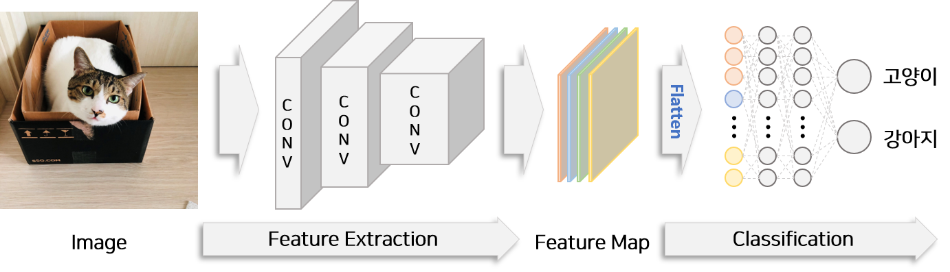
일반적인 이미지 분류 모델 구조 예시
- flatten 후 여러 층의 fc layer를 통과하면 위치 정보가 소실된다. 즉, CNN이 무엇을 보고 특정 class로 분류한 것인지 모르게 된다.
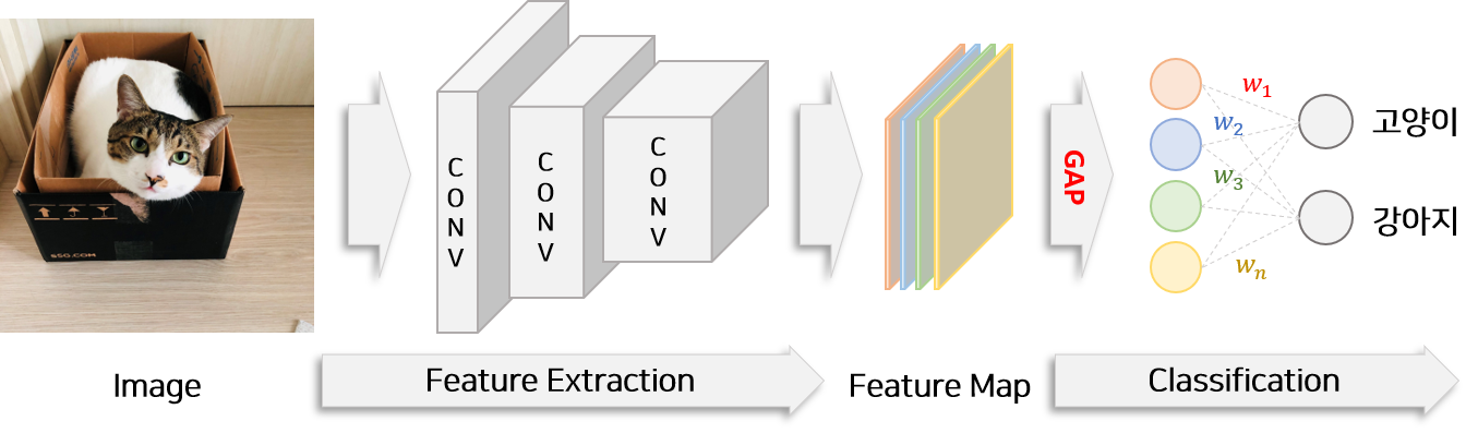
GAP가 적용된 이미지 분류 모델 구조 예시
- flatten 단계에서 Global average pooling 사용
- fully connected layer의 수를 줄이고 마지막 classification layer 하나만을 이용하여 모델을 구성.
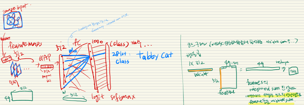
도식
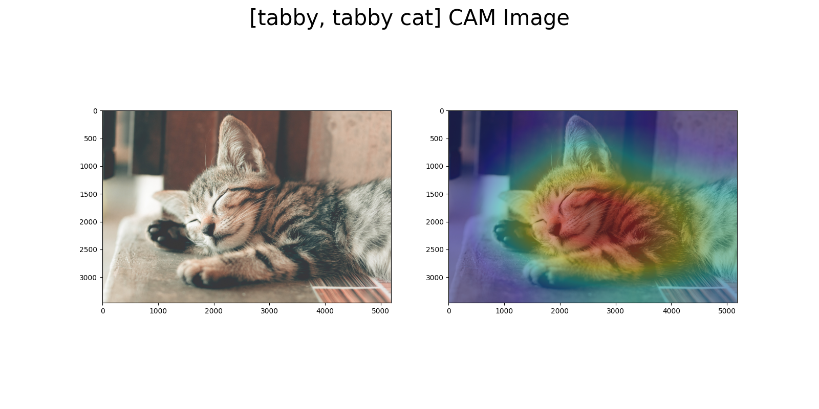
결과 이미지
###
장단점
- 장점:
- 단점:
- 기존 네트워크의 성능을 크게 저하시키지 않는다고 저자는 주장하지만, 떨어지긴 함
- 기존의 네트워크 구조를 변경해야 함. (FC Layer 제거)
- conv feature maps → global average pooling → softmax layer
- softmax layer 가기 전에 피처맵을 바로 얻어야해서, 특정 네트워크에서만 사용 가능하다.
- 극복 방안:
- 정확도: 피처 맵을 gradient signal과 합친 것, Grad-CAM
적용 방법(논문)
- 실험 대상 CNN 모델:
- AlexNet [10]
- VGGnet [23]
- GoogLeNet [24]
- 실험 설정:
- 각 모델에서 fully-connected 레이어를 제거하고, GAP(Global Average Pooling) 및 fully-connected softmax 레이어로 대체
- 마지막 GAP 이전의 컨볼루션 레이어의 공간 해상도를 조정하여 매핑 해상도 개선
- 네트워크 수정:
- AlexNet: conv5 이후의 레이어 제거하여 매핑 해상도 13 × 13
- VGGnet: conv5-3 이후의 레이어 제거하여 매핑 해상도 14 × 14
- GoogLeNet: inception4e 이후의 레이어 제거하여 매핑 해상도 14 × 14
- 네트워크 수정 및 Fine-tuning:
- 위의 각 네트워크에 3 × 3 크기, 스트라이드 1, 패딩 1을 가진 1024 개의 유닛을 가진 컨볼루션 레이어 추가
- 컨볼루션 레이어 뒤에 GAP 레이어와 softmax 레이어 추가
- ILSVRC [20]의 130만 개 훈련 이미지에서 1000-way object classification을 위해 fine-tuning 진행
- 최종 네트워크: AlexNet-GAP, VGGnet-GAP, GoogLeNet-GAP
- 비교 대상:
- 분류 작업: 원래의 AlexNet, VGGnet, GoogLeNet, Network in Network (NIN)
- 지역화 작업: 원래의 GoogLeNet, NIN, CAM 대신 역전파 사용
- 최대 풀링 대신 평균 풀링을 사용한 GoogLeNet 결과 (GoogLeNet-GMP)
- 평가:
- 분류 및 지역화를 위한 오류 메트릭스 (top-1, top-5) 사용
- 분류 작업: ILSVRC 검증 세트에서 평가
- 지역화 작업: 검증 세트와 테스트 세트에서 평가
Code
import torch
from torchvision import datasets, models, transforms
import torch.nn.functional as F
from PIL import Image
from matplotlib import pyplot as plt
import urllib.request
import ast
import numpy as np
import cv2

## 이미지 경로 설정
img_path = r'D:\GitHub_Project\koyumi0601.github.io\_posts\MachineLearning\Lecture_Legend13_Record\CAM_ClassActivationMap\cat.jpg'  # 분석할 이미지 파일 경로

## Resnet은 ImageNet에서 Training 되었으므로 image Net의 class 정보를 가져옵니다.
classes_url = 'https://gist.githubusercontent.com/yrevar/942d3a0ac09ec9e5eb3a/raw/238f720ff059c1f82f368259d1ca4ffa5dd8f9f5/imagenet1000_clsidx_to_labels.txt'

## class 정보 불러오기
with urllib.request.urlopen(classes_url) as handler:
    data = handler.read().decode()
    classes = ast.literal_eval(data)

## Resnet 불러오기
model_ft = models.resnet18(pretrained=True)
model_ft.eval()

## Imagenet Transformation 참조
## https://github.com/pytorch/examples/blob/42e5b996718797e45c46a25c55b031e6768f8440/imagenet/main.py#L89-L101

normalize = transforms.Normalize(mean=[0.485, 0.456, 0.406], std=[0.229, 0.224, 0.225])
preprocess = transforms.Compose([
    ## Resize는 사용하지 않고 원본을 추출
   transforms.Resize((224,224)),
   transforms.ToTensor(),
   normalize
])

## 그림을 불러옵니다.
raw_img = Image.open(img_path)

## 이미지를 전처리 및 변형
img_input = preprocess(raw_img)

## 모델 결과 추출
output = model_ft(img_input.unsqueeze(0))

## 클래스 추출
softmaxValue = F.softmax(output)
class_id=int(softmaxValue.argmax().numpy())

## Resnet 구조 참고
## https://github.com/pytorch/vision/blob/master/torchvision/models/resnet.py
def get_activation_info(self, x):
    # See note [TorchScript super()]
    x = self.conv1(x)
    x = self.bn1(x)
    x = self.relu(x)
    x = self.maxpool(x)
    x = self.layer1(x)
    x = self.layer2(x)
    x = self.layer3(x)
    x = self.layer4(x)
    return x

## Feature Map 추출
feature_maps = get_activation_info(model_ft, img_input.unsqueeze(0)).squeeze().detach().numpy()
## Weights 추출
activation_weights = list(model_ft.parameters())[-2].data.numpy()
## numpy로 이미지 변경
numpy_img = np.asarray(raw_img)

def show_CAM(numpy_img, feature_maps, activation_weights, classes, class_id):
    ## CAM 추출
    cam_img = np.matmul(activation_weights[class_id], feature_maps.reshape(feature_maps.shape[0], -1)).reshape(feature_maps.shape[1:])
    cam_img = cam_img - np.min(cam_img)
    cam_img = cam_img/np.max(cam_img)
    cam_img = np.uint8(255 * cam_img)

    ## Heat Map으로 변경
    heatmap = cv2.applyColorMap(cv2.resize(255-cam_img, (numpy_img.shape[1], numpy_img.shape[0])), cv2.COLORMAP_JET)

    ## 합치기
    result = numpy_img * 0.5 + heatmap * 0.3
    result = np.uint8(result)

    fig=plt.figure(figsize=(16, 8))
    ## 원본 이미지
    ax1 = fig.add_subplot(1, 2, 1)
    ax1.imshow(numpy_img)
    ## CAM 이미지
    ax2 = fig.add_subplot(1, 2, 2)
    ax2.imshow(result)
    plt.suptitle("[{}] CAM Image".format(classes[class_id]), fontsize=30)
    plt.show()

show_CAM(numpy_img, feature_maps, activation_weights, classes, class_id)
https://velog.io/@conel77/%EB%85%BC%EB%AC%B8%EB%A6%AC%EB%B7%B0Grad-CAM%EA%B3%BC-CAM-Class-activation-map
https://joungheekim.github.io/2020/09/29/paper-review/